A few tools to discover hidden data

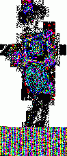
1. Limitations

I wrote these programs a while ago to help me in my exploration of steganography. Please note that they are very limited in scope. First, I use the very simple uncompressed flat 24-bits BMP image format as an example, because it's very easy to work with. These programs could be extended or adapted to other more complex formats. Second, I will focus here on one of the simplest steganography method (and so, the easiest to attack): sequential or linear use of the Least Significant Bit (LSB) of each pixel. Third, I will mainly talk about simple graphics with few colors, not photographic pictures.

There is no universal steganographic attack, just like there is no universal anti-virus tool (hint: I know that very well). If you suspect some file to contain hidden data, you will have to do some research, test several hypothesis, compare steganographic signatures with the ones of already analysed programs (another analogy with anti-virus technology), and probably code your own tools. This is just an example of what can be done in some particular cases. There is one example of a visual attack, and one example of a statistical attack.

The truth is that I think I've lost a little bit of interest in all of this. Or maybe I just don't have time anymore. Or maybe both. Anyway. As I had these programs sitting on my computer for a long time, I thought that maybe they could be of some interest for a handful of persons who are interested in the subject.

2. Visual attack: enhance LSBs

This very simple program was used to produce the images here, here and here. It's going to do the opposite of what a steganographical tool generally does. It will eliminate all 7 high-level bits for each pixel except the last LSB. So all bytes are going to be 0 or 1. The problem is that 0 or 1 on a 256 values range won't give any visible color. So, I enhance these LSBs. Basically, a 0 stays at 0, and a 1 becomes maximum value, or 255. That will give some flashy colors, the LSBs of the original image are going to become very visible, good enough for a visual check. So maybe we can see some patterns emerge.

The program and its source are here. Just run it, and select a 24-bits BMP file. An enhanced LSB image of the original image will be created in the same directory. Its name will be the same except that a "_LSB" extension will be added. That's it. Modify it freely to suit your needs. For example, you could enhance the second bit plane instead of the first one, or whatever you need.

Let's see an example with a random image sitting on my computer. It's the Beat Girl, the symbol of late 70's english ska band "The Beat". We will use one of the simplest free steganography tools available, InPlainView, without using the XOR encryption. To view as a web page, I re-transformed all the BMPs as GIFs. You can get the actual BMPs by clicking on the links below the images.

What is hidden	How the image looks like	How the enhanced LSBs look like	Comments
Nothing	original BMP	original BMP	We can see that the LSBs are very strange on this picture. I would guess these big blocks come from some JPG step before this image reached me. JPG works on 8x8 pixels blocks. Never use JPG for this kind of image. JPG is for photographs.
1 kb of random data	original BMP	original BMP	The random data hidden in the LSBs becomes very apparent. Note that the first line of pixels in the BMP file is the last line of the image on the screen, a peculiarity of the BMP format. This is why hidden LSBs appear in the bottom of the image.
5 kb of random data	original BMP	original BMP	Even more random "hidden" data.
Poem "If" by Rudyard Kipling, 1.5 Kb ASCII text	original BMP	original BMP	Now the hidden data is not random bytes but a simple text, we can see a pattern appearing in the enhanced LSBs. Something like vertical lines. It's due to a particularity of ASCII encoding. Most of the letters (especially similar ones, like the lower case group, which are the vast majority of a normal text) have many bits in common (3 out of 8 in the case of lower case). So you have a repeating pattern every 8 bits. In BMP pictures, you hide 3 bits in one pixel (one in the Red, one in the Green, one in the Blue). So you will see similar pixels appearing every ((8/3)x3) pixel, which is 8 pixels. That's what we see here: the vertical bands come back every 8 pixels. In conclusion, this very simple visual attack can give you an idea of not only the size of the hidden text, but also of its nature, just by looking at an image.

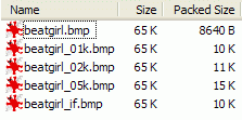
Now just for fun, another little simple experiment. Take the original BMPs above, with various things hidden inside, and compress them with your favorite packer. Then look at the size of the compressed images. Here is what I have with 7-Zip compressor, using the zip algorithm:

So, as you can see, these images look all the same and have the same size. Just looking at them, you cannot see any difference, and cannot guess there are different things hidden in them (well, that's the point of steganography). But when you compress them, the fact that something is hidden becomes apparent. Especially when you hide random data (or an encrypted message, which will look like random data). Random data does not compress, because it doesn't have any redundancy that compression algorithm use. So add 5 kb of random data in an image, you cannot see it because it is in the LSBs, but the compressed size of this image will be roughly 5 Kb higher than the original image, as we can see here.

My point here is that sometimes, what you cannot see by eye is not missed by mathematical algorithms. Which is a nice introduction for the next chapter.

3. Statistical attack: chi-square analysis

     3.1. Introduction

This statistical attack was published in 2000 by a german group led by Andreas Westfeld. I want to thank him first, because he took the time to reply to a few e-mails from me. The exact reference of this paper is: A. Westfeld and A. Pfitzmann, "Attack on Steganographic Systems", Lectures Notes in Computer Science, vol. 1768, Springer-Verlag, Berlin, 2000, pp. 61-75.. You can download the PDF from his site (check also this page, there is even a high-level language implementation in Java of this attack, with source code).

Please note that, since then, better and more reliable attacks have been published for sequential (or not) LSB embedding. For example, you may want to check the RS attack from Jessica Fridrich lab: J. Fridrich, M. Goljan, R. Du, "Reliable Detection of LSB Steganography in Color and Grayscale Images", 2002.

So why did I chose this particular attack if it's not the best one? Well, I have to admit something here: I'm extremely imcompetent when it comes to mathematics. And these academic papers are just that : mathematics. I just don't understand some of the formulas used. So I chose the older attack because, ahem, I could (almost) understand it, and code a tool to automatize it. Even more, to do mathematics in pure assembler is not the easiest thing in the world, but it's still fun.

This program and its source are available here.

     3.2. How does it work ?

So how does this attack work? Let's try to explain it in simple terms.

First, let's define the conditions. We have a simple image. I'm going to use again the 24-bits BMP format. As you can see above, the LSBs of this kind of image are not at all random. If you look at the Beat Girl without anything hidden, you see that there is a huge amount of similar background LSBs, all set to 1 (so it's white when you enhance them). And than big blocky zones of other LSBs, often black (so a lot of contiguous LSBs set to zero). So, nothing random at all.

The message we are going to hide in the LSBs of the image is the opposite: it's for example an encrypted text, so it's very random.

Let's take a simple example, hiding a random message in a zone of the image which has the same color everywhere. Let's say almost all black, to simplify. Before embedding the message, you will have almost all bytes at 0. All the LSBs will be at zero too. After embedding the random message, the LSBs will tend to be closer to a 50/50 distribution: half of the LSBs will be 0 and half will be 1. We call that a Pair of Values (PoV): the number of 1s and the number of 0s.

But we can go further than that. Instead of considering only the last bit (the LSB), we can take in account more bits, and still compare the Pair of Values to check if they are close to 50/50 distribution. Let's take an example with the 2 last bits. There are 4 possible values. So, 2 different Pair of Values. The Pair of values will differ only by the last bit:

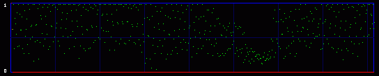
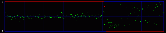
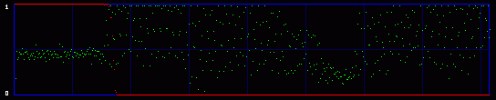
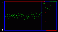
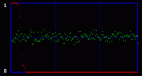
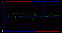
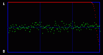
Now you get it. We are actually going to consider the whole 8 bits of each byte. So we will have 256 possible values, and 128 Pairs of Values.

So what kind of mathematics are we going to do on these 128 PoVs? Well, we first calculate them. So we have the measured frequency for each real (extracted from the image) Pair of Values. As an example, let's say that we will find, on a population of 500, 100 times the value 01011100 and 400 times the value 01011101. We construct a big table with these real values.

At the same time, we calculate the theorical frequency of the Pair of Values if they are represented randomly (ie if there is a random message embedded in the last LSB). It's easy: they should have a frequency of 50% each. So on the example above, the theorical values would be 250 times for the value the value 01011100, and 250 again for the value 01011101. We construct a second big table with these theorical values.

Then we compare these two tables of 128 PoVs with a chi-square test. You can find an explanation of this test in every basal-level book about statistics, much better than mine. Basically, this is to answer the following question: are these two populations (measured and theorical) significantly different? If they are significantly different, then the distribution of LSBs is not random: the probability is high that there is no hidden random message. If they are significantly close, then the distribution of LSBs is close to random: the probability is high that there is a hidden random message embedded in the LSBs.

This test is done in incremental parts of the BMP image. Each time we add more bytes, 128 seems to be good enough. So the first time the test is done from bytes 0 to 128. One value is outputted and plotted on a graph. Then we do the same test from bytes 0 to 256, and we output a second point of the curve. An so on.

     3.3. First example

Okay, you can admit you didn't understand a thing on the above paragraphs. Me neither anyway.

So let's do practical examples. My program will output a graph with two curves. The first one in red is the result of the chi-square test. If it's close to one, than the probability for a random embedded message is high. The second output is a simple idea I had, to add another layer of verification: it's the average value of the LSBs on the current block of 128 bytes. So, if there is a random message embedded, this green curve will stay around 0.5. On the graph network, every vertical blue line represents 1 kilobyte of embedded data.

As this output graph will not be saved (I was just lazy to add this routine), you may want to do a screenshot if you want to keep it.

Lets check the output of the Beat Girl images above. We get this:

What is hidden	Output result
Nothing
1 Kb random data
5 kb random data
"If" Poem, 1.5 Kb ASCII text

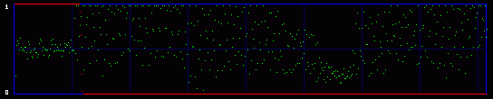
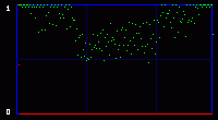
So what do we see? First, there is a little bit more than 8 vertical zones. Which means that we can hide a little bit more than 8 kb of data. Why? Because the Beat Girl image is 98x225 pixels. One pixel can be used to hide three bits (one in the LSB of each RGB color tone). So we can hide (98x225)x3 bits. To get the number of kilobytes, we divide by 8 and by 1024: ((98x225)x3)/(8x1024). Well, that should be around 8.1 kilobytes.

Than, let's look at the curves. On the first output, coming from the Beat Girl without embedded data, the chi-square red output is flat at zero all along the picture: there is nothing hidden. The green average of LSBs is very variable, sometimes very close to 1, and sometimes very close to 0. Curiously, it goes down clearly after around 5.5 kilobytes of data. Guess were it is on the image. It's the horizontal zone between the two hands, where there is no white background: a lot of LSBs are black in this zone, so, close to 0.

Now let's look at the second one. The red curve stays at maximum at the beginning, than suddenly drops to zero once we reach one kilobyte of hidden data. We can conclude that there is a hidden message of one kilobyte. Look at how the green average in this first kilobyte of hidden data is much more packed around 0.5. Another good sign of randomness.

It's the same with the next one, the image with 5 Kb of hidden data. The red curve drops immediately after reaching the fifth kilobyte vertical blue mark.

It seems that in such a non-random image, even a text is considered random by comparison. That's probably why the output is able to clearly detect the embedded 1.5 kb poem.

     3.4. Second example

Just for fun, because I actually used a lot the Google various logos for my experiments. And I loved the one they did for the birthday of Piet Mondrian, an artist I appreciate very much (ever wondered why I only use primary colors?). So I will use it, with its size reduced by half so I can put everything on the same line.

Hidden	Image	Enhanced LSBs	Chi-Square
Nothing	BMP	BMP
2 kb random data	BMP	BMP

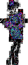
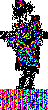
Once again, the presence of 2 kb of hidden data is very visible with both attacks, visual and statistical.

     3.5. Third example

Now you may say: why do we need this output when the embedded data is so clearly visible in the first visual attack in chapter 2? It's because sometimes, a visual attack is not enough, and you need to rely on mathematics to detect small changes that you cannot see by eye. Let's take an example with another image. It may be a particular case. As I said before, this chi-square attack, at least in my hands, does not work very well for many photographs. But here is an example that works, for the sake of the demonstration.

The crazy-looking running guy on the picture is me, somewhere in a New Hampshire field, trying to catch back one of my returning boomerangs.

Hidden	Image	Enhanced LSBs	Chi-Square
Nothing	BMP	BMP
1 kb random data	BMP	BMP
2 kb random data	BMP	BMP

This time, the visual attack is of no use. As we can see on the three enhanced LSB images, there is no detectable difference. No pattern appearing. Everything look random. So here we reach the limit of a visual attack. We need to use statistical analysis.

Even the green curve of the average of LSBs cannot tell us anything. There is no evident break.

But the red curve, the output of the chi-square analysis, shows some difference. It can see something that we cannot see. Statistical detection is more sensitive than our eyes, and I guess that was my final point.

Just for the sake of writing a little bit more boring stuff, we can notice something that often happens in my experiments with photographs: there is a sort of latency in the red curve. Even without hidden data, it starts at maximum and stays like that for some time. It's close to a false positive. It looks like the LSB in these images are very close to random, and the algorithm needs a large population (remember the analysis is done on an incrementing population of pixels) before reaching a threshold where it can decide that actually, they are not random after all, and the red curve starts to go down. The same sort of latency happens with hidden data. You hide 1 or 2 kb, but the red curve does not go down right after this amount of data. It waits a little bit, here respectively at around 1.3 kb and 2.6 kb.

4. Conclusion

The two attacks I show above are old and simple. They were designed for a simple kind of steganography. In just a few years, there seem to have been many more subtle and powerful attacks on a larger set of steganography algorithms. I've read a few recent papers, and even if I don't understand one tenth of the underlying mathematical concepts, I was impressed by the apparent power of these new ways to do steganalysis. And this published academic work may very well be only the tip of the iceberg. As many (unproven) rumors talked about the use of steganography by the Evil Terrorists™, you can be sure that some people may work on that subject, and they are not the type that publish scientific papers.

So, once again, don't believe people who claim that steganography is undetectable. Especially their own secret algorithm that they will try to sell you, claiming that it has "military grade" and is of "world-class strength", "unbreakable even by the NSA". Ask them for a proof. Even better, crack their algorithm yourself.

And that's it for today.

Have a nice day!